Matplotlib also does not have a function that takes histograms and fit them. The following is my simple solution to do a gaussian fit on a 1D histogram that exists as a Numpy array.

from scipy.optimize import curve_fit

def gaus(x, a, mu, sig):
  return a * np.exp(-0.5 * np.square((x - mu) / sig))

def fit_gaus(hist, edges, mu=0.0, sig=1.0):
  hist = hist.astype(np.float64)
  edges = edges.astype(np.float64)
  xdata = (edges[1:] + edges[:-1]) / 2
  ydata = hist
  popt, pcov = curve_fit(gaus, xdata, ydata, p0=[np.max(hist), mu, sig])
  if not np.isfinite(pcov).all():
    raise RuntimeError("Fit has failed to converge.")
  popt[2] = np.abs(popt[2])  # take absolute value of sigma
  return popt

In Matplotlib, you can use hist and hist2d to make 1D & 2D histograms. These functions take unbinned data as input, do the binning, and then plot the histograms. (They are based on Numpy histogram and histogram2d.) In HEP, we often work directly with binned data (i.e. histograms), but there is no available function in Matplotlib that takes histograms and plot them.

I found that the rootpy project has implemented methods to plot ROOT histograms using Matplotlib. For example, this uses Matplotlib hist2d to plot a ROOT 2D histogram.

Based on the example, I wrote some simple functions that take binned data that exist as a Numpy array and plot it using Matplotlib hist or hist2d.

def hist_on_binned_data(hist, edges, ax=None, **kwargs):
  from matplotlib.pyplot import gca
  if ax is None:
    ax = gca()
  x = (edges[1:] + edges[:-1]) / 2
  h, edges, patches = ax.hist(x, weights=hist, bins=edges, **kwargs)
  return (h, edges, patches)

def hist2d_on_binned_data(hist, xedges, yedges, colorbar=False, ax=None, **kwargs):
  from matplotlib.pyplot import gca
  if ax is None:
    ax = gca()
  xdata = (xedges[1:] + xedges[:-1]) / 2
  ydata = (yedges[1:] + yedges[:-1]) / 2
  xv, yv = np.meshgrid(xdata, ydata)
  x = xv.ravel()
  y = yv.ravel()
  z = hist.T.ravel()
  h, xedges, yedges, image = ax.hist2d(x, y, weights=z, bins=(xedges, yedges), **kwargs)
  if colorbar:
    cb = ax.figure.colorbar(image, ax=ax)
  return (h, xedges, yedges, image)

To change the CSS style in a Jupyter notebook, simply create a cell at the top with the styles:

%%html
<style>
.rendered_html p {font-size: 16px;}
</style>

To apply the CSS style to all the notebooks, create the file ~/.jupyter/custom/custom.css and add the styles there.

The transverse impact parameter of a track, $d_{0}$, is determined by the vector product of $\vec{r} \times \vec{p}$, where $\vec{r}$ is the transverse displacement vector of the point of closest approach (PCA) w.r.t the origin $(0,0)$, and $\vec{p}$ is the transverse momentum vector of the track at the PCA. For a straight track with $p_{\mathrm{T}} = \infty$, $d_{0}$ with the correct sign can be obtained from the following equation:

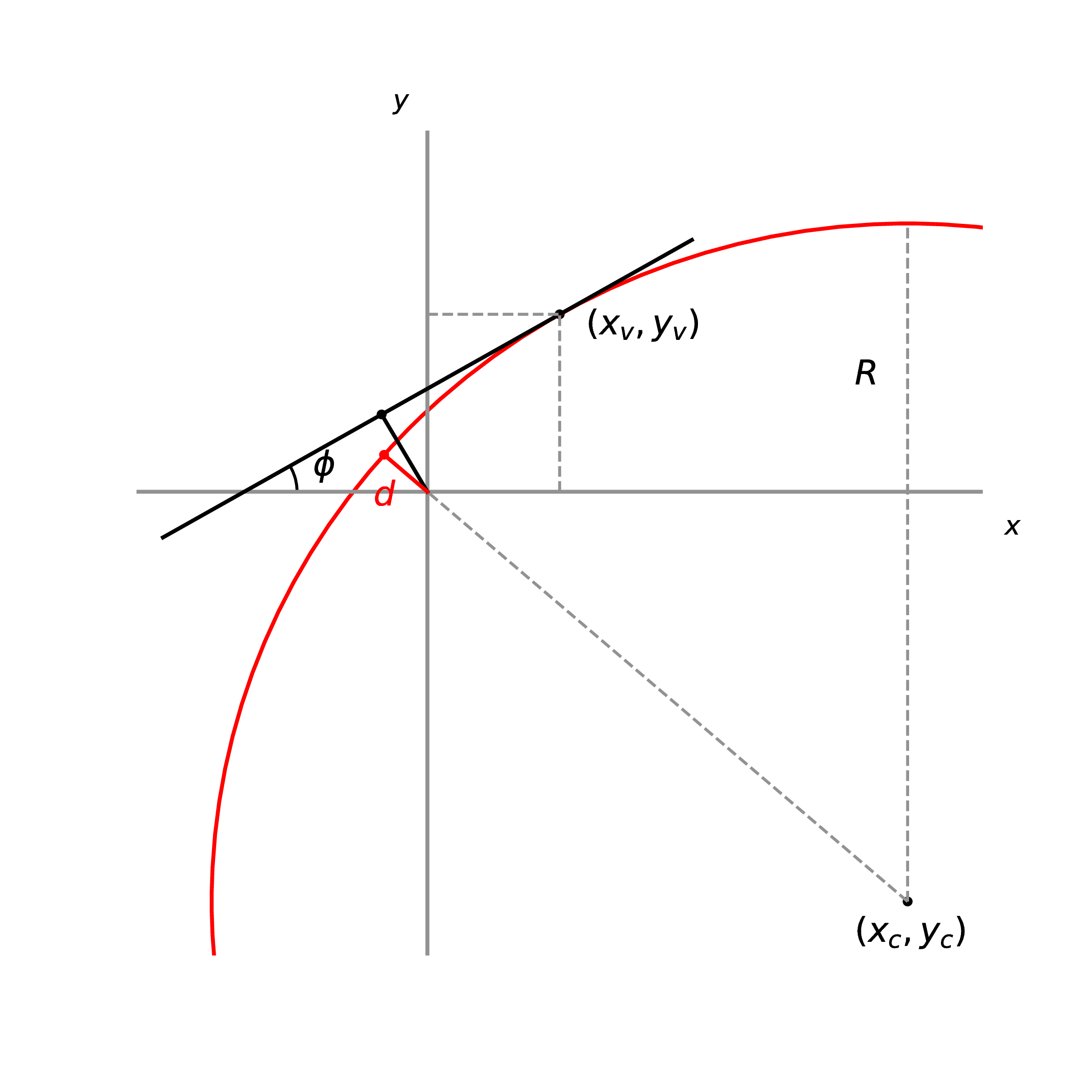
where $\phi$ is the azimuth angle of the track momentum, $(x_{v}, y_{v})$ is the location of the production vertex.

But tracks are curved, and we cannot always approximate a curve with a straight line. To calculate the $d_{0}$ for a curved track, firstly we define the signed radius of curvature $R$:

where $p_{\mathrm{T}}$ is the transverse momentum in GeV/c, $q$ is the charge of the track, $B$ is the magnetic field in Tesla, and $R$ is in cm. The constant 0.003 is the speed of light multiplied by the necessary conversion factors. The negative sign accounts for the fact that a track with negative charge rotates counter-clockwise, i.e. $\phi(r)$ increases as $r$ increases, so $R$ is positive.

The exact equation for $d_{0}$ can be obtained from the following equation:

where $(x_{c}, y_{c})$ is the center of the track circle. It is related to $(x_{v}, y_{v})$ by:

Since $\operatorname{sign}(R) = -q$, the equation can also be written more clearly as:

from which we can see that the length of $d_{0}$ is given by the difference between the center of the track circle and the radius of the track curvature. The following figure shows the relationship between $d_{0}$, $R$, and $(x_{c}, y_{c})$.

Moreover, at the point of closest approach, the momentum $\phi$ is tangential to the $\phi_{\text{PCA}}$:

Given $d_{0}$ and momentum $\phi$ at the PCA, $(x_{\text{PCA}}, y_{\text{PCA}})$ can be found using:

Charged tracks in a uniform magnetic field in the barrel geometry follow the track equations:

where $R = \frac{p_{\mathrm{T}}}{0.003 B}$, $R$ and $r$ are in cm and $B$ is the magnetic field in Tesla. The constant 0.003 is the speed of light multiplied by the necessary conversion factors. A muon with $p_{\mathrm{T}} = 2~\text{GeV}$ in the CMS experiment ($B = 3.8~\text{T}$) has $R = 1.75~\text{m}$.

In the endcap geometry, the track equations are:

where $R \cot{\theta} = \frac{p_{\mathrm{z}}}{0.003 B}$, $z$ is in cm. By the way, $\cot{\theta}$ can be easily calculated from $\eta$ via the equation $\cot{\theta} = \sinh(\eta)$.

When considering a vertex-unconstrained fit, with transverse impact parameter $d_{0} \neq 0$, the $\phi_{r}$ equation becomes:

For the endcap muon trigger in CMS, one has to take into account several considerations:

• Detector planes perpendicular (instead of parallel) to the solenoid magnetic field;
• Significant multiple scattering;
• Significant energy loss;
• Neutron background;
• Non-uniform magnetic field, including a non-zero radial component.