Moving average in Batch Normalization

In TensorFlow/Keras Batch Normalization, the exponential moving average of the population mean and variance are calculated as follows:

moving_mean = moving_mean * momentum + batch_mean * (1 - momentum)
moving_var = moving_var * momentum + batch_var * (1 - momentum)

where momentum is a number close to 1 (default is 0.99). In the actual code, the moving average are updated in a more efficient way:

moving_mean -= (moving_mean - batch_mean) * (1 - momentum)
moving_var -= (moving_var - batch_var) * (1 - momentum)

They are equivalent as shown below ($\mu$ is the moving mean, $\mu_{B}$ is the batch mean, $\alpha$ is the momentum):

\[\begin{align} \mu &= \alpha\mu + (1 - \alpha) \mu_{B} \\ &= \mu - (1 - \alpha) \mu + (1 - \alpha) \mu_{B} \\ &= \mu - (1 - \alpha) (\mu - \mu_{B}) \end{align}\]

Hence, the moving average will decay by the difference between the existing value and the new value, multiplied with a decay factor of (1 - momentum). A lower value of momentum means that older values are forgotten sooner. This results in a faster-changing moving average.


Huber and logcosh loss functions

Huber loss is like a “patched” squared loss that is more robust against outliers. For small errors, it behaves like squared loss, but for large errors, it behaves like absolute loss:

\[\operatorname{Huber}(x) = \begin{cases} \frac{1}{2}{x^2} & \text{for } |x| \le \delta, \\ \delta |x| - \frac{1}{2}\delta^2 & \text{otherwise.} \end{cases}\]

where $\delta$ is an adjustable parameter that controls where the change occurs.

Recently, I encountered the logcosh loss function in Keras: $\operatorname{logcosh}(x) = \log(\cosh(x))$. 
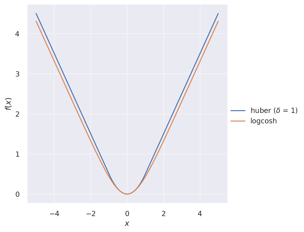
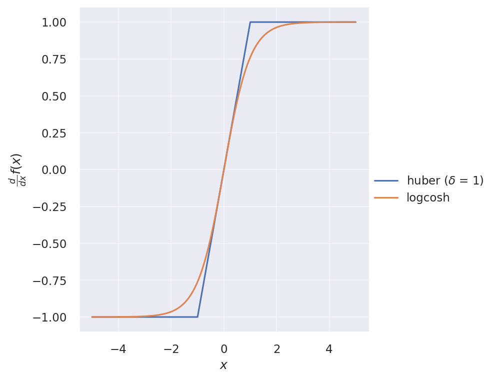
It looks very similar to Huber loss, but twice differentiable everywhere. Its first derivative is simply $\tanh(x)$. The two loss functions are illustrated below:

And their gradients:

One has to be careful about numerical stability when using logcosh. Instead of the original expression, we can write $\cosh(x)$ in terms of exponentials as $\cosh(x) = \frac{e^x + e^{-x}}{2}$, and define logcosh as follows:

import numpy as np

logcosh = lambda x: np.logaddexp(x, -x) - np.log(2)

Both the loss functions are available in TensorFlow/Keras: 1, 2. But I did an implementation of Huber loss on my own before it was added to Keras. For posterity’s sake, here is my own implementation:

from tensorflow.python.keras import backend as K
from tensorflow.python.framework import constant_op
from tensorflow.python.ops import array_ops
from tensorflow.python.ops import math_ops

def huber(y_true, y_pred, delta=1.345):
  delta = constant_op.constant(delta, dtype=y_pred.dtype)
  half = constant_op.constant(0.5, dtype=y_pred.dtype)
  abs_error = math_ops.abs(math_ops.subtract(y_pred, y_true))
  squared_loss = half * math_ops.squared_difference(y_pred, y_true)
  absolute_loss = delta * abs_error - half * math_ops.square(delta)
  return K.mean(array_ops.where_v2(abs_error < delta, squared_loss, absolute_loss), axis=-1)

Also, here’s my own implementation of logcosh using $\cosh(x) = \frac{1 + e^{-2x}}{2 e^{-x}}$ for positive $x$ and $\cosh(x) = \frac{e^{2x} + 1}{2 e^x}$ for negative $x$ to ensure numerical stability. The softplus activation function $\operatorname{softplus}(x) = \log(1 + e^{x})$ is used in the calculation.

from tensorflow.python.keras import backend as K
from tensorflow.python.framework import constant_op
from tensorflow.python.ops import array_ops
from tensorflow.python.ops import nn_ops

def logcosh(y_true, y_pred):
  double = constant_op.constant(2.0, dtype=y_pred.dtype)
  log_two = constant_op.constant(np.log(2.0), dtype=y_pred.dtype)
  zeros = array_ops.zeros_like(y_pred, dtype=y_pred.dtype)
  error = math_ops.subtract(y_pred, y_true)
  positive_branch = nn_ops.softplus(-double * error) + error - log_two
  negative_branch = nn_ops.softplus(double * error) - error - log_two
  return K.mean(array_ops.where_v2(error < zeros, negative_branch, positive_branch), axis=-1)

Fun fact, softplus can be generalized as follows according to this Quora answer:

\[f_{t}(x) = \frac{1}{t} \log\left(1 + e^{tx}\right)\]

where $t = 1$ yields the softplus activation function, while $t \to \infty$ yields the ReLU activation function. Note that softplus is differentiable everywhere while ReLU is not differentiable at $x = 0$.

\[\begin{align} f_{1}(x) &= \operatorname{softplus}(x) = \log(1 + e^{x}) \\ f_{\infty}(x) &= \operatorname{ReLU}(x) = \max(0, x) \end{align}\]

How to cast to NumPy arrays

This post is written for people like me who can never remember how to convert an array-like object back to a NumPy array. An array-like object refers to the following (not an exhaustive list):

  • pandas: DataFrame
  • tensorflow: Tensor
  • h5py: Dataset
  • dask: Array

General

If you don’t want to look up the answers on StackOverflow, just try: np.array(). There is a good chance that it will work.

import numpy as np
import pandas as pd
df = pd.DataFrame({"A": [1, 2], "B": [3, 4]})
arr = np.array(df)
print(arr.__class__)
# <class 'numpy.ndarray'>

Pandas

The recommended way to convert a pd.DataFrame to np.ndarray is to_numpy().

import pandas as pd
arr = pd.DataFrame({"A": [1, 2], "B": [3, 4]}).to_numpy()
print(arr.__class__)
# <class 'numpy.ndarray'>

TensorFlow

For TensorFlow v2 in the eager mode, use numpy() to convert a tf.Tensor (it must be of type EagerTensor).

import tensorflow as tf
x = tf.constant([[1, 2],
                 [3, 4]])
arr = x.numpy()
print(arr.__class__)
# <class 'numpy.ndarray'>

h5py

You can slice a h5py.Dataset with an empty tuple (i.e. ()) to get a np.ndarray. Actually, any supported slicing operations should return a np.ndarray.

import h5py
f = h5py.File('dummy.h5', 'w')
dset = f.create_dataset('dset', (10,10,10), 'f')
arr = dset[()]
print(arr.__class__)
# <class 'numpy.ndarray'>
arr = dset[:]
print(arr.__class__)
# <class 'numpy.ndarray'>

Dask

Dask arrays are lazy. To convert it into a NumPy array, a Dask array needs to be computed via the compute() method.

import dask
import dask.array as da
x = da.ones(10, chunks=(5,))
arr = x.compute()
print(arr.__class__)
# <class 'numpy.ndarray'>
y = da.ones(10, chunks=(5,))
arr0, arr1 = dask.compute(x, y)
print(arr0.__class__, arr1.__class__)
# <class 'numpy.ndarray'> <class 'numpy.ndarray'>

As a footnote, to convert a scalar np.ndarray back to a built-in Python object, use item(). For instance, np.array([1]).item() will return 1.


Running Python tasks in parallel

There are many options to run Python tasks in parallel. This provides a brief description for some of the options.

  • threading and multiprocessing are part of the standard library. threading is used for thread-based parallelism, while multiprocessing is used for process-based parallelism. If your tasks involve Python objects that lock the Global Interpreter Lock (GIL), then threading does not provide much parallelism, and you should opt for multiprocessing. On the other hand, if your tasks involve NumPy objects that release the GIL, then threading is a better choice. In general, threading has less overheads compared to multiprocessing.

  • concurrent.futures is also part of the standard library. It provides a high-level interface for asynchronous parallelism (using Future objects). You can easily choose between a “thread” pool or a “process” pool by using ThreadPoolExecutor or ProcessPoolExecutor. If you are running user-level codes, I believe concurrent.futures is usually the best option. But if you are writing more low-level codes, I believe you still want to choose between threading or multiprocessing. Note that you can still use threads from multiprocessing by using multiprocessing.pool.ThreadPool.

  • dask is a powerful library that helps with the common pains dealing with large data and parallel computing (e.g. delayed, lazy loading, array chunking, distributed computing). There are two kinds of schedulers: the single-machine scheduler (default) and the more advanced dask.distributed. The advanced dask.distributed provides asynchronous parallelism similar to concurrent.futures and can be used on a cluster. But if you are just running codes on a single machine, the default scheduler should suffice (it requires zero setup). You can set the scheduler to “threads”, “processes” or “single-threaded”. The Best Practices pages (1, 2, 3) contain some very useful examples.

  • joblib is a lightweight library that also provides lazy evaluation and parallel computing. For process-based parallelism, it uses the alternative serialization library cloudpickle instead of pickle, which allows you to serialize more things.

I want to mention that Keras and Tensorflow also have built-in parallelism. So, if you are dealing with ML stuff, you should be able to use what is offered by Keras/Tensorflow (e.g. keras.Model.fit). However, I think the documentation is kind of difficult to go through.

Simple code snippets:

def fun(x):
  return x * x

# No parallelism
result = map(fun, range(10))

# Using concurrent.futures
import concurrent.futures
with concurrent.futures.ProcessPoolExecutor(max_workers=4) as executor:
  result = executor.map(fun, range(10))

# Using multiprocessing
import multiprocessing
with multiprocessing.Pool(processes=4) as pool:
  result = pool.imap(fun, range(10))

# Using threads from multiprocessing
with multiprocessing.pool.ThreadPool(processes=4) as pool:
  result = pool.imap(fun, range(10))

Proper colormaps

Proper colormaps for scientific plots (not rainbow!):

References: