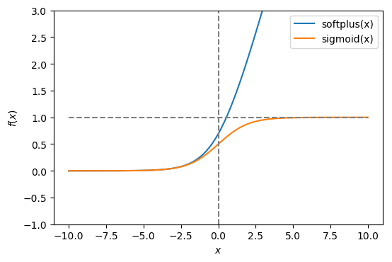
The softplus function is a smooth approximation to the ReLU activation function, and is sometimes used in the neural networks in place of ReLU.
\[\operatorname{softplus}(x) = \log(1 + e^{x})\]
It is actually closely related to the sigmoid function. As $x \to -\infty$, the two functions become identical.
\[\operatorname{sigmoid}(x) = \frac{1}{1 + e^{-x}}\]
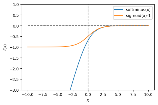
The softplus function also has a relatively unknown sibling, called softminus.
\[\operatorname{softminus}(x) = x - \operatorname{softplus}(x)\]
As $x \to +\infty$, it becomes identical to $\operatorname{sigmoid}(x) - 1$. In the following plots, you can clearly see the similarities between softplus & softminus and sigmoid.
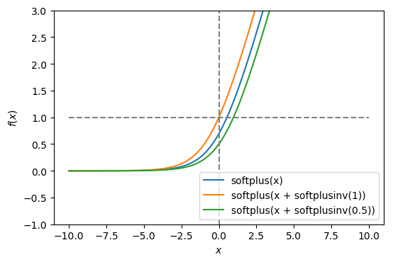
Furthermore, there is also an inverse softplus function that does the transformation $x = \operatorname{softplusinv}(\operatorname{softplus}(x))$.
\[\operatorname{softplusinv}(x) = \log(e^{x} - 1)\]
Using $\operatorname{softplusinv}(x)$ as an additive constant allows you to adjust the $y$-intercept of the softplus function. For instance, $\operatorname{softplus}(x + \operatorname{softplusinv}(1))$ returns a function with $y$-intercept = 1.
The inverse of the sigmoid function is called logit. As such, $x = \operatorname{logit}(\operatorname{sigmoid}(x))$.
\[\operatorname{logit}(p) = \log\left(\frac{p}{1-p}\right)\]
As these functions involve $\exp(x)$ and $\log(x)$, sometimes you might run into numerical stability issues. For instance, this happens to $\exp(x)$ when $x$ is too large; for $\log(x)$ when $x$ is close to zero. The following are the safer expressions of softplus and softminus that should help avoid those issues.
\[\operatorname{softplus}(x) = \max(0, x) + \log(1 + e^{-|x|})\]
\[\operatorname{softminus}(x) = \min(0, x) - \log(1 + e^{-|x|})\]
While for the sigmoid function, you can simply call the hyperbolic tangent function, because $\tanh(x)$ is just a scaled $\operatorname{sigmoid}(x)$.
\[\operatorname{sigmoid}(x) = \frac{1}{2} \left[1 + \tanh\left(\frac{x}{2}\right)\right]\]
As a reminder, $\tanh(x)$ is defined as:
\[\tanh(x) = \frac{e^x - e^{-x}}{e^x + e^{-x}} = \frac{1 - e^{-2x}}{1 + e^{-2x}}\]
All these functions are easily written with NumPy.
import numpy as np

softplus = lambda x: np.log1p(np.exp(x))

softminus = lambda x: x - softplus(x)

sigmoid = lambda x: 1 / (1 + np.exp(-x))

one_minus_sigmoid = lambda x: 1 / (1 + np.exp(x))

logit = lambda x: np.log(x) - np.log1p(-x)

softplusinv = lambda x: np.log(np.expm1(x))

softminusinv = lambda x: x - np.log(-np.expm1(x))

safe_softplus = lambda x: x * (x >= 0) + np.log1p(np.exp(-np.abs(x)))

safe_softminus = lambda x: x * (x < 0) - np.log1p(np.exp(-np.abs(x)))

safe_sigmoid = lambda x: 0.5 * (1 + np.tanh(0.5 * x))

safe_one_minus_sigmoid = lambda x: 0.5 * (1 + np.tanh(0.5 * -x))
Softplus is also used to compute the log probabilities used in the binary cross-entropy loss function.
\[\operatorname{log prob}_{1}(x) = \log(p(x)) = -\operatorname{softplus}(-x)\]
\[\operatorname{log prob}_{0}(x) = \log(1-p(x)) = -\operatorname{softplus}(x)\]
The subscripts “0” and “1” are the class labels, and $p(x)$ is the probability of being class “1”. Substitute $p(x) = \operatorname{sigmoid}(x)$ to get the above results. The following plot shows the log prob curves.
