Huber and logcosh loss functions
Huber loss is like a “patched” squared loss that is more robust against outliers. For small errors, it behaves like squared loss, but for large errors, it behaves like absolute loss:
\[\operatorname{Huber}(x) = \begin{cases} \frac{1}{2}{x^2} & \text{for } |x| \le \delta, \\ \delta |x| - \frac{1}{2}\delta^2 & \text{otherwise.} \end{cases}\]where $\delta$ is an adjustable parameter that controls where the change occurs.
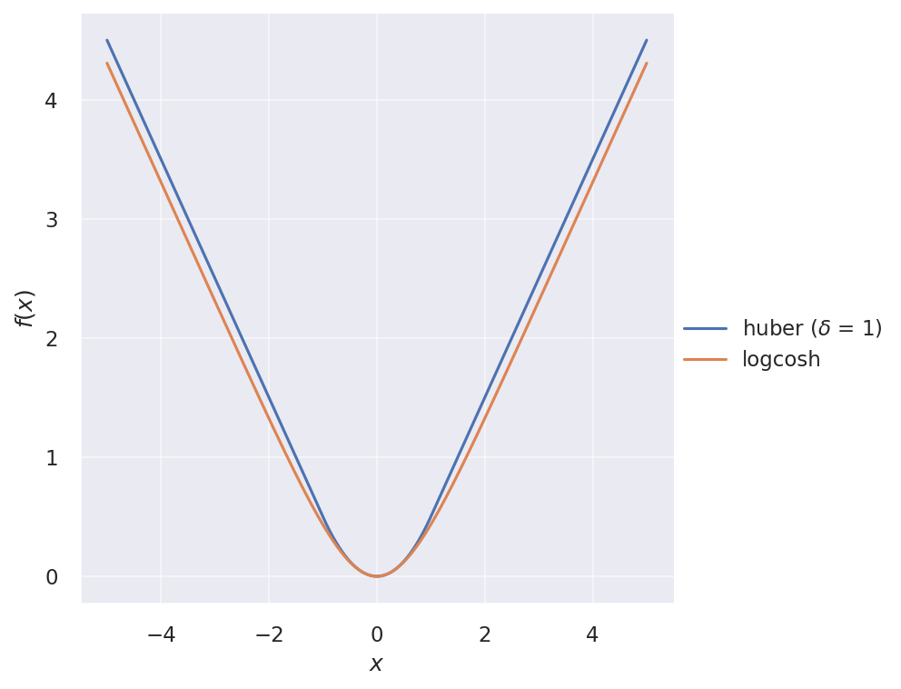
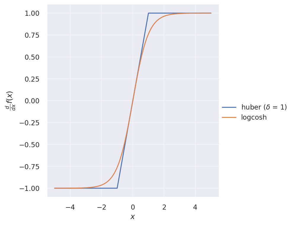
Recently, I encountered the logcosh loss function in Keras: $\operatorname{logcosh}(x) = \log(\cosh(x))$. It looks very similar to Huber loss, but twice differentiable everywhere. Its first derivative is simply $\tanh(x)$. The two loss functions are illustrated below:

And their gradients:

One has to be careful about numerical stability when using logcosh. Instead of the original expression, we can write $\cosh(x)$ in terms of exponentials as $\cosh(x) = \frac{e^x + e^{-x}}{2}$, and define logcosh as follows:
import numpy as np

logcosh = lambda x: np.logaddexp(x, -x) - np.log(2)
Both the loss functions are available in TensorFlow/Keras: 1, 2. But I did an implementation of Huber loss on my own before it was added to Keras. For posterity’s sake, here is my own implementation:
from tensorflow.python.keras import backend as K
from tensorflow.python.framework import constant_op
from tensorflow.python.ops import array_ops
from tensorflow.python.ops import math_ops

def huber(y_true, y_pred, delta=1.345):
  delta = constant_op.constant(delta, dtype=y_pred.dtype)
  half = constant_op.constant(0.5, dtype=y_pred.dtype)
  abs_error = math_ops.abs(math_ops.subtract(y_pred, y_true))
  squared_loss = half * math_ops.squared_difference(y_pred, y_true)
  absolute_loss = delta * abs_error - half * math_ops.square(delta)
  return K.mean(array_ops.where_v2(abs_error < delta, squared_loss, absolute_loss), axis=-1)
Also, here’s my own implementation of logcosh using $\cosh(x) = \frac{1 + e^{-2x}}{2 e^{-x}}$ for positive $x$ and $\cosh(x) = \frac{e^{2x} + 1}{2 e^x}$ for negative $x$ to ensure numerical stability. The softplus activation function $\operatorname{softplus}(x) = \log(1 + e^{x})$ is used in the calculation.
from tensorflow.python.keras import backend as K
from tensorflow.python.framework import constant_op
from tensorflow.python.ops import array_ops
from tensorflow.python.ops import nn_ops

def logcosh(y_true, y_pred):
  double = constant_op.constant(2.0, dtype=y_pred.dtype)
  log_two = constant_op.constant(np.log(2.0), dtype=y_pred.dtype)
  zeros = array_ops.zeros_like(y_pred, dtype=y_pred.dtype)
  error = math_ops.subtract(y_pred, y_true)
  positive_branch = nn_ops.softplus(-double * error) + error - log_two
  negative_branch = nn_ops.softplus(double * error) - error - log_two
  return K.mean(array_ops.where_v2(error < zeros, negative_branch, positive_branch), axis=-1)
Fun fact, softplus can be generalized as follows according to this Quora answer:
\[f_{t}(x) = \frac{1}{t} \log\left(1 + e^{tx}\right)\]where $t = 1$ yields the softplus activation function, while $t \to \infty$ yields the ReLU activation function. Note that softplus is differentiable everywhere while ReLU is not differentiable at $x = 0$.
\[\begin{align} f_{1}(x) &= \operatorname{softplus}(x) = \log(1 + e^{x}) \\ f_{\infty}(x) &= \operatorname{ReLU}(x) = \max(0, x) \end{align}\]